How to interpret the normal distribution?
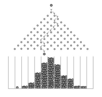
Let’s take a look at the Galton Machine. You may have seen this in somewhere, such as the New York Hall of Science or the Children’s Discovery Museum of San Jose. The inventor was Sir Francis Galton who was a Mathematician in 19th century. When the balls are dropped from the center top of the machine, each of them goes through a random trajectory, as at each pinpoint in their trajectories they make a random turn either towards left or right with equal probability. Eventually, all the balls fall into one-ball-wide bins at the bottom. The height of ball columns accumulated in the bins seems to follow a bell curve, reminding us the normal distribution.
The outcome of this experiment of dropping massive amounts of balls in the Bean Machine is very stable. The stability of the bell shape implies that something systematic actually emerge from the seemly stochastic process of ball dropping. This something systematic is further revealed as the normal distribution (aka Gaussian distribution), which is one of the major foundations of statistics. Sometimes it seems everything just converge to normal distribution, as many of the theories and models in our textbooks and academic articles have shown.
Is this a coincidence? Or does this imply there is something structural, that determines its manifestation in real-world representations?
Mathematics … Articulates Our Understanding
The stability of the outcome of the Galton machine is no accidence. We could perform a rigorous analysis to identify its articulated form – a mathematical construct that admits an explicit analytic structure.
The first step to conduct an analytic inquiry is always challenging, since you need to know what question to ask. As a matter of fact, most times when we feel unsure or unknow of something, we are in the stage of what we don’t know about what we don’t know. It would be much easier if we have known what we don’t know – that usually means to get the solution of the problem what matters is investment of time and resource. But in the stage of what we don’t know about what we don’t know, we need to gain more insights of the system and experience many errors and failures to finally achieve our success.
Fortunately, we could learn much from existing works about the analysis of the Galton machine. We have learned the probability distribution. The outcome of the Galton machine admits the form as a probability distribution, if we define the column of final arrival as a random variable$X$. So our first question is, what is the mathematical details of this probability distribution.
We have learned that, to define a probability distribution function, we need the sample space first. Here, let’s say there are $n$ columns. We could label the columns from left to right as $0,1,2,\cdots,n$, which form our sample space.
Then the next question is to determine specifics of this probability distribution. We may ask, what is the probability that a ball ends up in the column $k$?
It seems that there are many possible trajectories that the ball could take to arrive in column $k$. If we enumerate all the possible trajectories, we could try to determine the probability of each trajectory and then aggregate them together. However, this could be a very tedious effort.
There is an easier route to take – instead of asking how many possible trajectories a ball could take to arrive in column $k$, you may have noticed that the total number of turns a ball would make in order to reach the bottom is fixed as n. And more importantly, the outcome of where is the final definition depends on how many right turns (or left turns) the ball made during the trajectory, so the order of the turns doesn’t matter. For example, we don’t have to know what exactly order of the turns, but the simple knowledge of 8 right turns are made could tell us that the ball will end up in column $k=8$. Similarly, if we are told that the ball made 6 right turns, that means the ball ended up in column $k=6$.
Thus, the next question is to ask, what is the probability of the ball takes $k$ right turns? In total, there are n turns. For each turn, the probability of going right is the same – denoted as $p$. Then we could derive that the probability of $X=k$ as
$$ P(X=k)={n \choose k} p^k(1-p)^{n-k}, $$
where ${n \choose k}=\frac{n!}{k!(n-k)!}$. This is known as the Binomial distribution.
Now let’s further articulate the mathematical form by considering the extreme case that n goes to infinity.
To do so, we need to use the Stirling’s formula:
$$ n!\sim\sqrt{2\pi n}(\frac{n}{e})^n, $$
then we can obtain the result as:
$$ \lim_{n\to\infty}{n \choose k}p^k(1-p)^{n-k}\cong\frac{1}{\sqrt{2\pi np(1-p)}}e^{-\frac{(k-np)^2}{2np(1-p)}} $$
Remember that for binomial distribution, the mean $\mu=np$and the variance $\sigma^2=np(1-p)$. We can rewrite $\frac{1}{\sqrt{2\pi np(1-p)}}e^{-\frac{(k-np)^2}{2np(1-p)}}$ as $\frac{1}{\sqrt{2\pi \sigma}}e^{-\frac{(k-\mu)^2}{2\sigma^2}}$, which is the form of normal distribution!
Share on: